Physiological Data Analysis

Author

Enrico Toffalini

Published

February 11, 2025

Raw Data

Dataset inspect

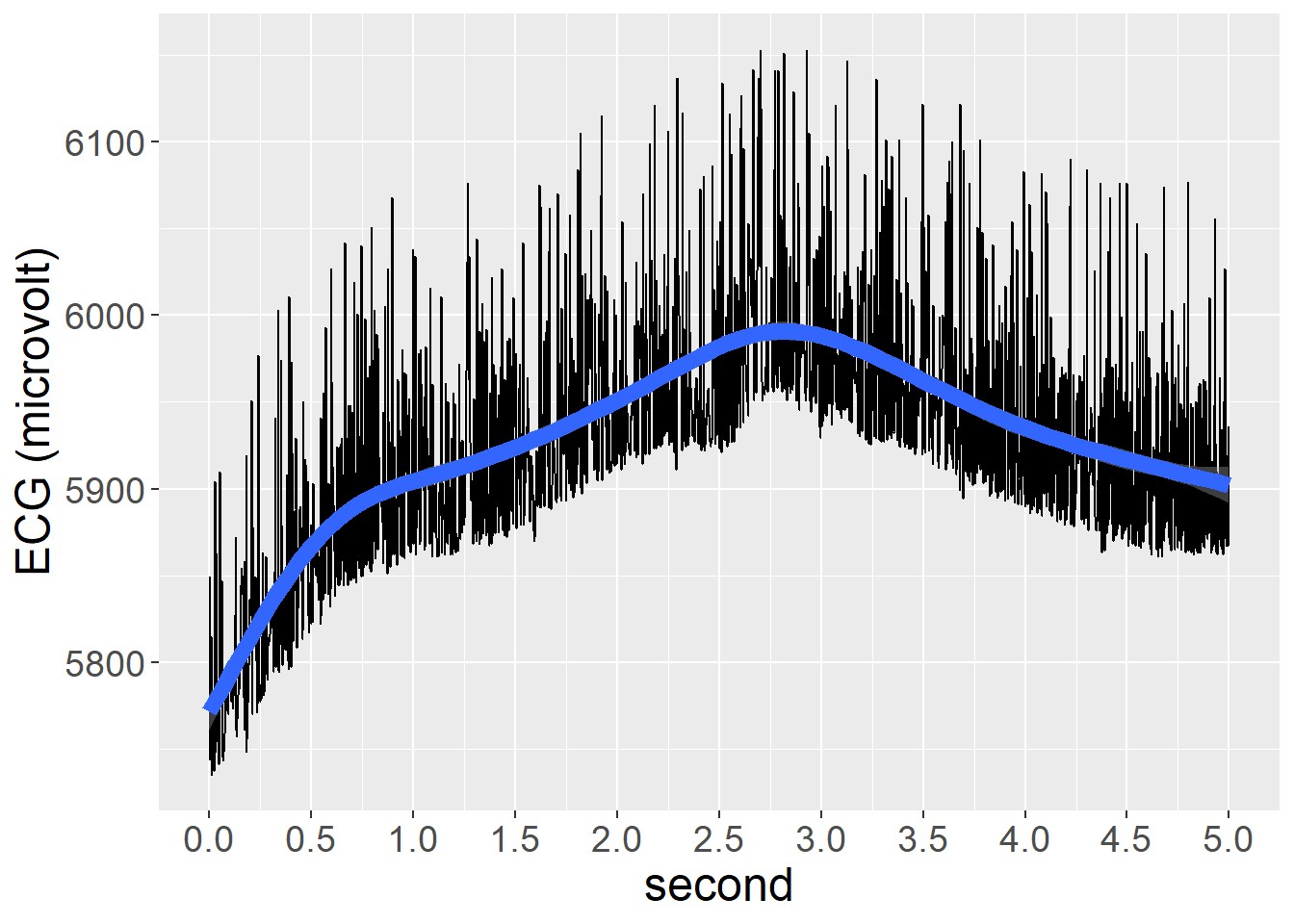
head(phy_raw_sample)

  row        ID second   ECG  EDA
1   0 Pilot_003  0.000 32396 5743
2   1 Pilot_003  0.002 32456 5849
3   2 Pilot_003  0.004 32484 5791
4   3 Pilot_003  0.006 32452 5815
5   4 Pilot_003  0.008 32432 5775
6   5 Pilot_003  0.010 32530 5735

Plot ECG sample (first 5 seconds)

Exercise: Based on the plot below, could you provide an estimate of beats per minute?

Show the code

library(ggplot2)

ggplot(phy_raw_sample[1:2500,],aes(x=second,y=ECG))+
  geom_line()+
  scale_x_continuous(breaks=seq(0,100,.5))+
  theme(text=element_text(size=18))+
  ylab("ECG (microvolt)")

Plot EDA sample (first 5 seconds), with a gam smoother

Show the code

ggplot(phy_raw_sample[1:2500,],aes(x=second,y=EDA))+
  geom_line()+
  scale_x_continuous(breaks=seq(0,100,.5))+
  geom_smooth(linewidth=3)+
  theme(text=element_text(size=18))+
  ylab("ECG (microvolt)")

Processed Data

Dataset inspect

phy[1:10,]

   ID Order Condition Minute HR       SCR
1   4   NNP   Resting      1 86 18.483025
2   4   NNP   Resting      2 87 11.945870
3   4   NNP   Resting      3 89 14.445035
4   4   NNP   Resting      4 87 13.538947
5   4   NNP   Resting      5 88  7.804276
6   4   NNP  Negative      1 90 10.097523
7   4   NNP  Negative      2 93 12.065430
8   4   NNP  Negative      3 89 12.116706
9   4   NNP  Negative      4 89 18.211881
10  4   NNP  Negative      5 90 15.136771

Heart Rate (HR)

HR visualization - by subject

ggplot(phy,aes(x=Minute,y=HR,color=Condition))+
  geom_line(aes(x=Minute,y=HR,group=paste0(ID,Condition)),alpha=.6,linewidth=1)+
  theme(text=element_text(size=18))+
  ylab("HR (bpm)")

HR visualization - aggregated and smoothed

ggplot(phy,aes(x=Minute,y=HR,color=Condition,fill=Condition))+
  geom_smooth(alpha=.2,linewidth=2)+
  theme(text=element_text(size=18))+
  ylab("HR (bpm)")

Statistical models on HR

Due to serious convergence issues, I cannot enter a full random effects formula, so results must be taken with caution.

fit_hr_Multiplicative = glmmTMB(
  HR ~ Minute * Condition + (1|ID),
  dispformula = ~ Condition,
  data = phy
)
fit_hr_Additive = glmmTMB(
  HR ~ Minute + Condition + (1|ID),
  dispformula = ~ Condition,
  data = phy
) 

anova(fit_hr_Multiplicative, fit_hr_Additive)

Data: phy
Models:
fit_hr_Additive: HR ~ Minute + Condition + (1 | ID), zi=~0, disp=~Condition
fit_hr_Multiplicative: HR ~ Minute * Condition + (1 | ID), zi=~0, disp=~Condition
                      Df    AIC    BIC  logLik deviance  Chisq Chi Df
fit_hr_Additive       10 4331.6 4377.6 -2155.8   4311.6              
fit_hr_Multiplicative 13 4334.1 4393.9 -2154.0   4308.1 3.4912      3
                      Pr(>Chisq)
fit_hr_Additive                 
fit_hr_Multiplicative     0.3219

# see summary of model coefficients
summary(fit_hr_Additive)

 Family: gaussian  ( identity )
Formula:          HR ~ Minute + Condition + (1 | ID)
Dispersion:          ~Condition
Data: phy

     AIC      BIC   logLik deviance df.resid 
  4331.6   4377.6  -2155.8   4311.6      728 

Random effects:

Conditional model:
 Groups   Name        Variance Std.Dev.
 ID       (Intercept) 137.7    11.73   
 Residual                NA       NA   
Number of obs: 738, groups:  ID, 37

Conditional model:
                  Estimate Std. Error z value Pr(>|z|)    
(Intercept)        79.6742     1.9950   39.94   <2e-16 ***
Minute              0.2059     0.0968    2.13   0.0334 *  
ConditionNeutral   -4.7535     0.4663  -10.19   <2e-16 ***
ConditionPositive  -4.4162     0.5194   -8.50   <2e-16 ***
ConditionNegative  -4.1819     0.4940   -8.47   <2e-16 ***
---
Signif. codes:  0 '***' 0.001 '**' 0.01 '*' 0.05 '.' 0.1 ' ' 1

Dispersion model:
                  Estimate Std. Error z value Pr(>|z|)    
(Intercept)         3.4761     0.1171  29.696  < 2e-16 ***
ConditionNeutral   -1.4153     0.1896  -7.466 8.28e-14 ***
ConditionPositive  -0.6098     0.1647  -3.702 0.000214 ***
ConditionNegative  -0.9317     0.1762  -5.288 1.24e-07 ***
---
Signif. codes:  0 '***' 0.001 '**' 0.01 '*' 0.05 '.' 0.1 ' ' 1

# plot predicted effects
plot(allEffects(fit_hr_Additive))

Skin Conductance Response (SCR)

SCR visualization - by subject

ggplot(phy,aes(x=Minute,y=SCR,color=Condition))+
  geom_line(aes(x=Minute,y=SCR,group=paste0(ID,Condition)),alpha=.6,linewidth=1)+
  theme(text=element_text(size=18))+
  ylab("SCR (microsiemens)")

There are extreme outlier observations! Let’s remove them:

phy$SCR[phy$SCR>600] = NA
ggplot(phy,aes(x=Minute,y=SCR,color=Condition))+
  geom_line(aes(x=Minute,y=SCR,group=paste0(ID,Condition)),alpha=.6,linewidth=1)+
  theme(text=element_text(size=18))+
  ylab("SCR (microsiemens)")

SCR visualization - aggregated and smoothed

ggplot(phy,aes(x=Minute,y=SCR,color=Condition,fill=Condition))+
  geom_smooth(alpha=.2,linewidth=2)+
  theme(text=element_text(size=18))+
  ylab("SCR (microsiemens)")

Statistical models on SCR

fit_scr_Multiplicative = glmmTMB(
  SCR ~ Minute * Condition + (1|ID),
  dispformula = ~ Condition,
  family = gaussian(link="log"),
  data = phy
)
fit_scr_Additive = glmmTMB(
  SCR ~ Minute + Condition + (1|ID),
  dispformula = ~ Condition,
  family = gaussian(link="log"),
  data = phy
) 

anova(fit_scr_Multiplicative, fit_scr_Additive)

Data: phy
Models:
fit_scr_Additive: SCR ~ Minute + Condition + (1 | ID), zi=~0, disp=~Condition
fit_scr_Multiplicative: SCR ~ Minute * Condition + (1 | ID), zi=~0, disp=~Condition
                       Df    AIC    BIC  logLik deviance  Chisq Chi Df
fit_scr_Additive       10 7614.8 7660.7 -3797.4   7594.8              
fit_scr_Multiplicative 13 7613.4 7673.0 -3793.7   7587.4 7.4002      3
                       Pr(>Chisq)  
fit_scr_Additive                   
fit_scr_Multiplicative    0.06018 .
---
Signif. codes:  0 '***' 0.001 '**' 0.01 '*' 0.05 '.' 0.1 ' ' 1

# see summary of model coefficients
summary(fit_scr_Additive)

 Family: gaussian  ( log )
Formula:          SCR ~ Minute + Condition + (1 | ID)
Dispersion:           ~Condition
Data: phy

     AIC      BIC   logLik deviance df.resid 
  7614.8   7660.7  -3797.4   7594.8      715 

Random effects:

Conditional model:
 Groups   Name        Variance Std.Dev.
 ID       (Intercept) 0.5196   0.7208  
 Residual                 NA       NA  
Number of obs: 725, groups:  ID, 37

Conditional model:
                  Estimate Std. Error z value Pr(>|z|)    
(Intercept)        3.59500    0.15378  23.377  < 2e-16 ***
Minute            -0.06922    0.01898  -3.647 0.000266 ***
ConditionNeutral   0.26327    0.08207   3.208 0.001337 ** 
ConditionPositive  0.61723    0.07030   8.779  < 2e-16 ***
ConditionNegative  0.22050    0.08367   2.635 0.008402 ** 
---
Signif. codes:  0 '***' 0.001 '**' 0.01 '*' 0.05 '.' 0.1 ' ' 1

Dispersion model:
                  Estimate Std. Error z value Pr(>|z|)    
(Intercept)         7.1011     0.1158   61.35  < 2e-16 ***
ConditionNeutral    0.4776     0.1738    2.75 0.005991 ** 
ConditionPositive   0.6139     0.1634    3.76 0.000173 ***
ConditionNegative   0.5448     0.1689    3.23 0.001256 ** 
---
Signif. codes:  0 '***' 0.001 '**' 0.01 '*' 0.05 '.' 0.1 ' ' 1

# plot predicted effects
plot(allEffects(fit_scr_Additive))

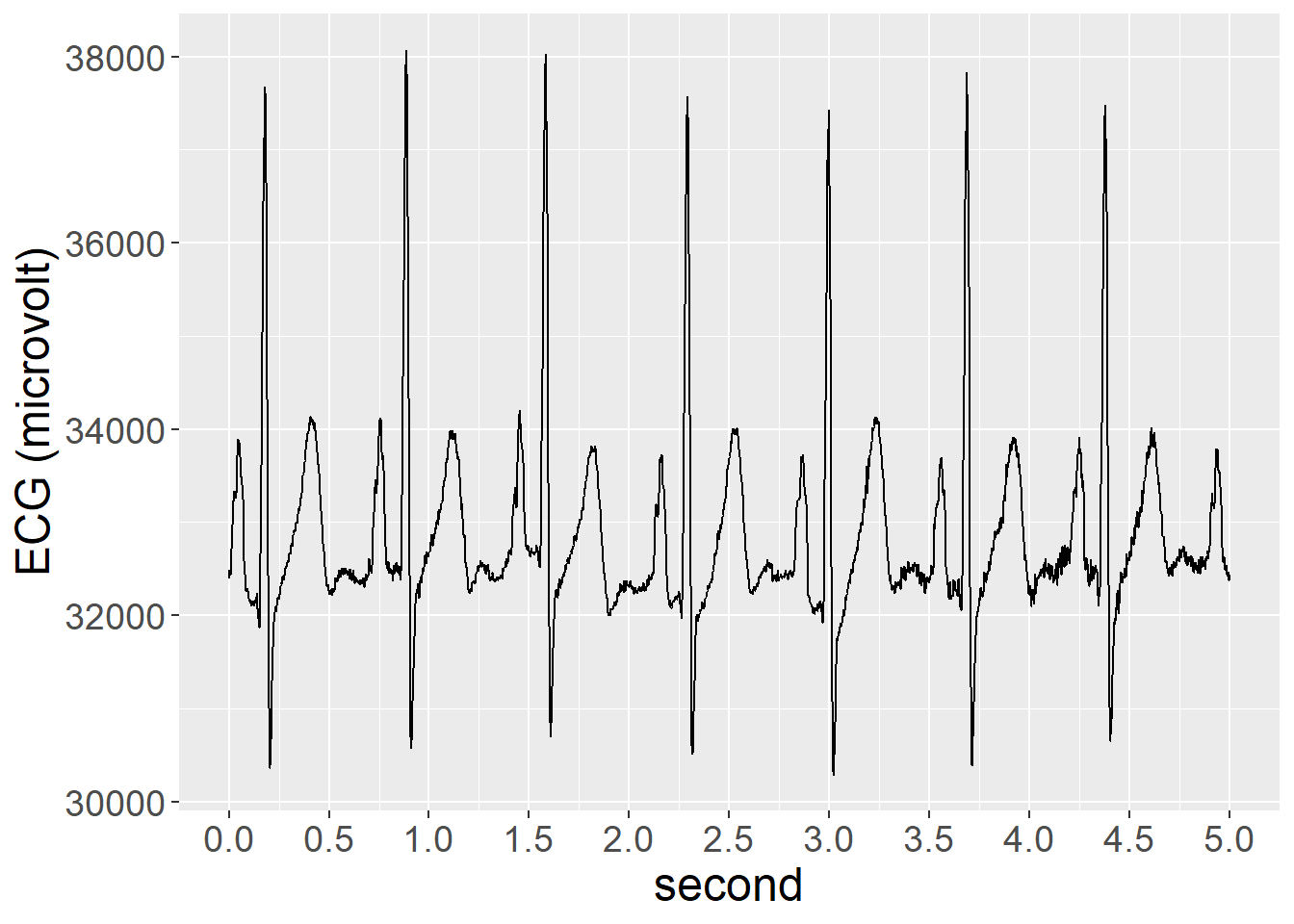
Comments and Conclusions

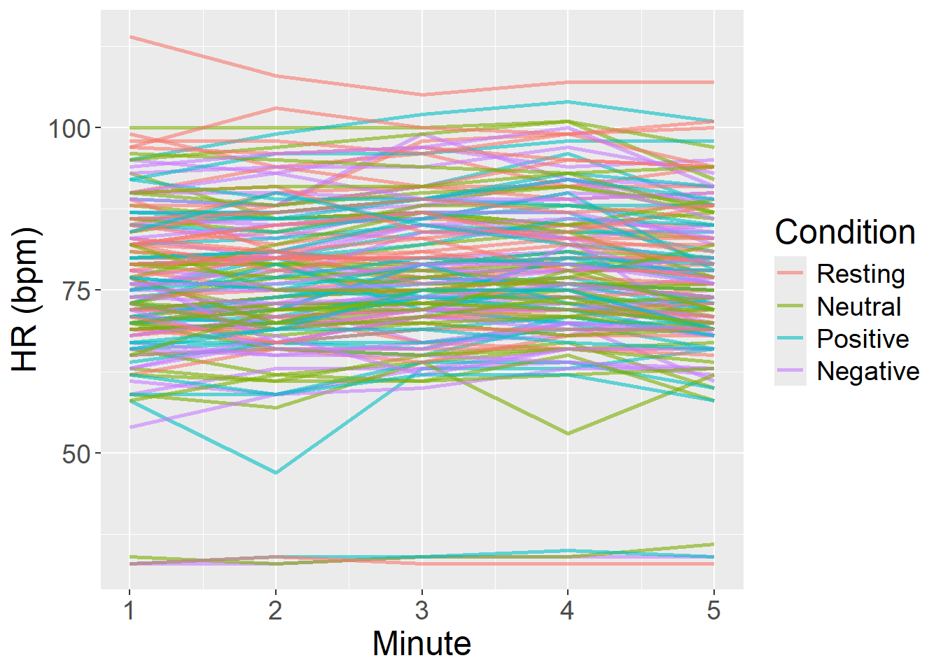
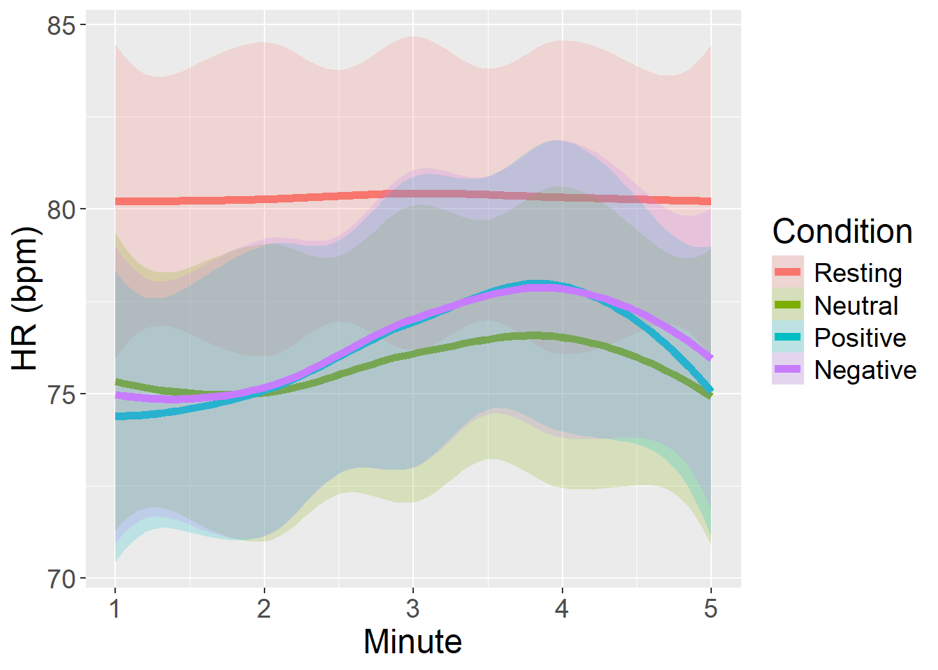
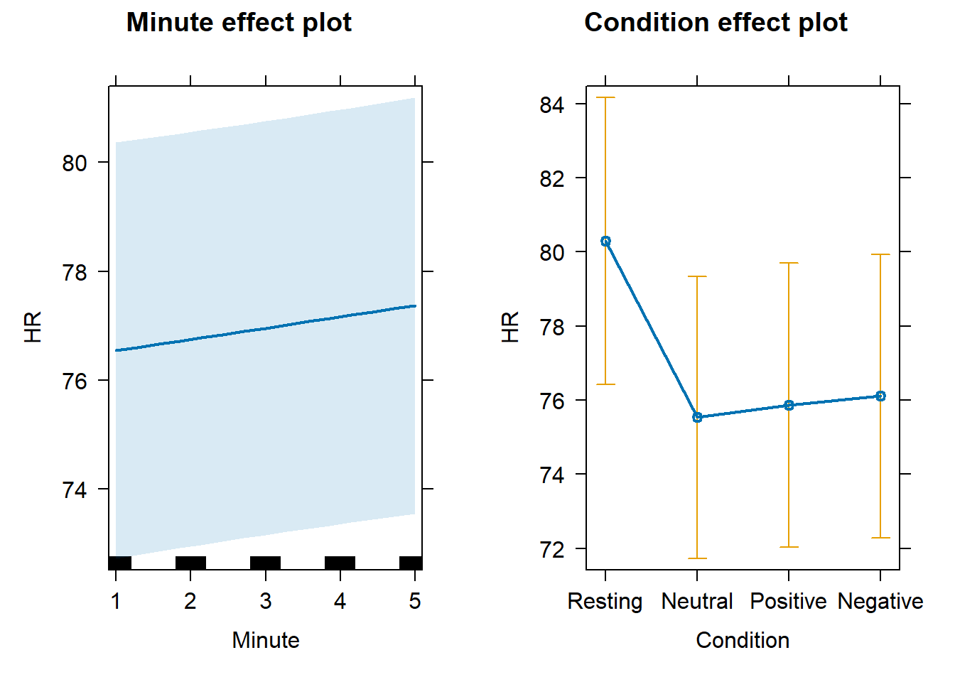
For Heart Rate, we observed highest mean values (and highest dispersion of scores) during the Resting state, while there were no relevant changes across the Neutral, Positive, or Negative video conditions, somehow unexpectedly. There was a slight tendency for HR to increase across time, independently from Condition.
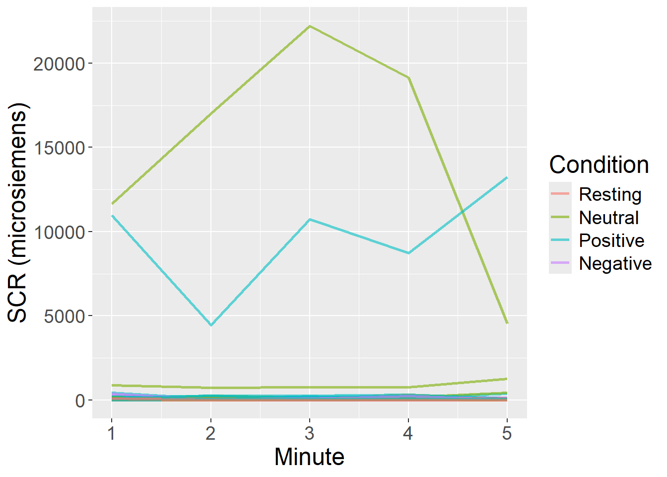
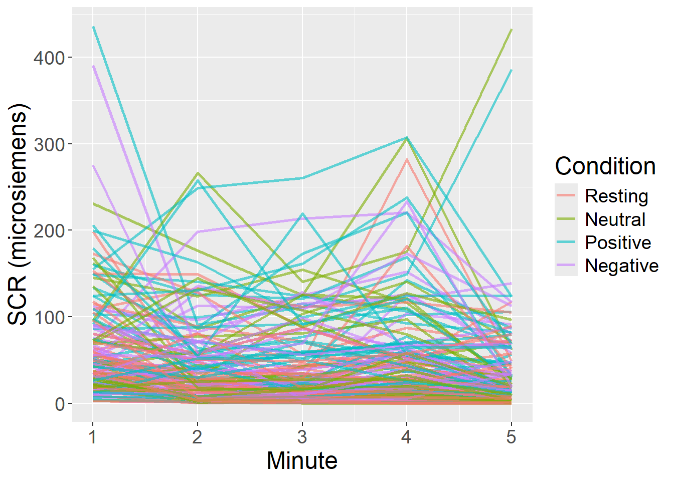
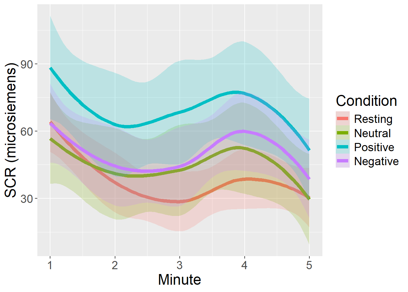
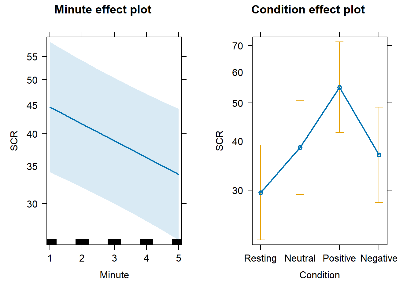
For Skin Conductance Response, we observed highest mean values during the Positive video condition, followed by Negative and Neutral conditions, with Resting state presenting the lowest values. Dispersion of scores also followed this patter. SCR also tended to reduce across time within each Condition, and quite independently from Condition.