Behavioral Data Analysis

Author

Enrico Toffalini

Published

February 11, 2025

Inspect Datasets

Let’s see the first few rows of each dataset for figuring out their structures. Note that Emotion varies within-subject.

head(ft)

  ID Order  Emotion PrePost Trial ITI
1  4   NNP Positive     Pre     1 993
2  4   NNP Positive     Pre     2 206
3  4   NNP Positive     Pre     3 171
4  4   NNP Positive     Pre     4 154
5  4   NNP Positive     Pre     5 169
6  4   NNP Positive     Pre     6 169

head(tp)

  ID Order  Emotion Retro_Estimate Prosp_Estimate
1  4   NNP Positive            6.5          51089
2  4   NNP  Neutral            5.0          85090
3  4   NNP Negative            4.0          65048
4  5   PNN Positive            7.0          56634
5  5   PNN  Neutral            6.0          58890
6  5   PNN Negative            7.0          90949

Finger Tapping

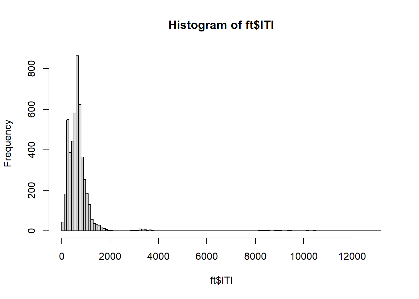
As recommended, let’s remove the first trial for each subject. Then, let’s inspect the distribution of ITI.

ft = ft[ft$Trial != 1, ]
ft = ft[ft$PrePost == "Post", ]
hist(ft$ITI, breaks=100)

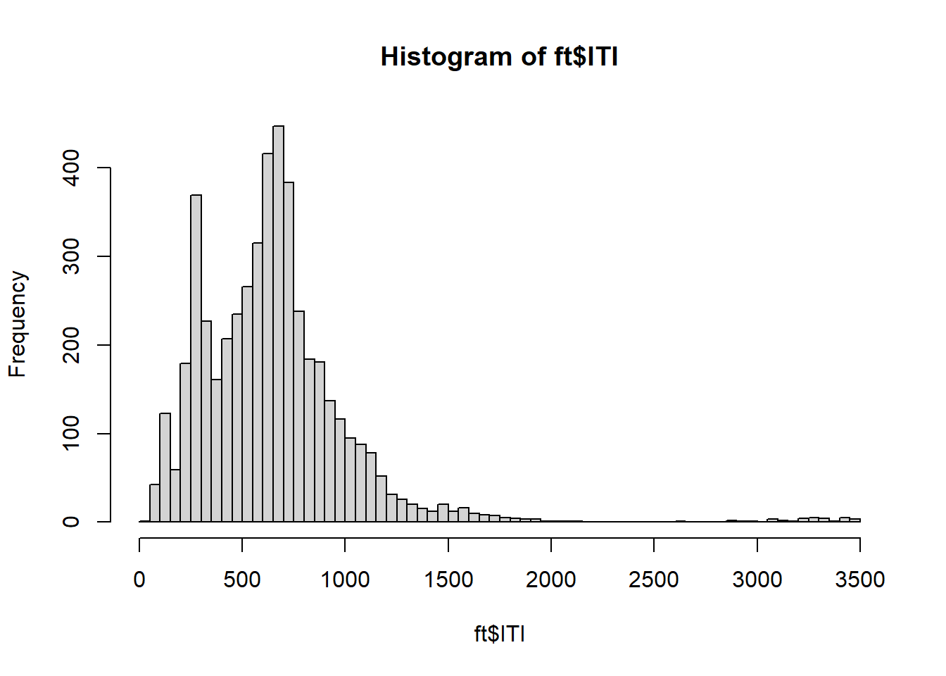
OUCH! There are a few outliers! Let’s remove ITI observations that are too far away from the average:

ITI_zScore = (ft$ITI - mean(ft$ITI))/sd(ft$ITI)
ft = ft[!abs(ITI_zScore) > 3, ]
hist(ft$ITI, breaks=100)

Fit Statistical Model on Finger Tapping

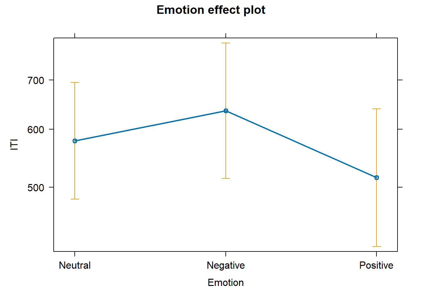
Because each participant provides multiple responses, we can test not only if Emotion affects average ITI, but also if it affects its dispersion. Let’s run a special model for this:

# prepare factorial variables
ft$ID = factor(ft$ID)
ft$Emotion = factor(ft$Emotion, levels=c("Neutral","Negative","Positive"))

# actually fit the model
fit_ft = glmmTMB(
  ITI ~ Emotion + (Emotion||ID),
  dispformula = ~ Emotion ,
  data = ft,
  family = Gamma(link="log")
)

# see summary of model coefficients
summary(fit_ft)

 Family: Gamma  ( log )
Formula:          ITI ~ Emotion + (Emotion || ID)
Dispersion:           ~Emotion
Data: ft

     AIC      BIC   logLik deviance df.resid 
 54458.6  54516.9 -27220.3  54440.6     4820 

Random effects:

Conditional model:
 Groups Name            Variance Std.Dev. Corr      
 ID     (Intercept)     0.3202   0.5659             
        EmotionNegative 0.1089   0.3300   0.00      
        EmotionPositive 0.1275   0.3571   0.00 0.00 
Number of obs: 4829, groups:  ID, 37

Conditional model:
                Estimate Std. Error z value Pr(>|z|)    
(Intercept)      6.36044    0.09307   68.34   <2e-16 ***
EmotionNegative  0.09439    0.05514    1.71   0.0869 .  
EmotionPositive -0.11543    0.05884   -1.96   0.0498 *  
---
Signif. codes:  0 '***' 0.001 '**' 0.01 '*' 0.05 '.' 0.1 ' ' 1

Dispersion model:
                Estimate Std. Error z value Pr(>|z|)    
(Intercept)      4.43535    0.03551  124.91  < 2e-16 ***
EmotionNegative -0.16648    0.05046   -3.30  0.00097 ***
EmotionPositive -0.04293    0.05013   -0.86  0.39181    
---
Signif. codes:  0 '***' 0.001 '**' 0.01 '*' 0.05 '.' 0.1 ' ' 1

# plot predicted effects
plot(allEffects(fit_ft))

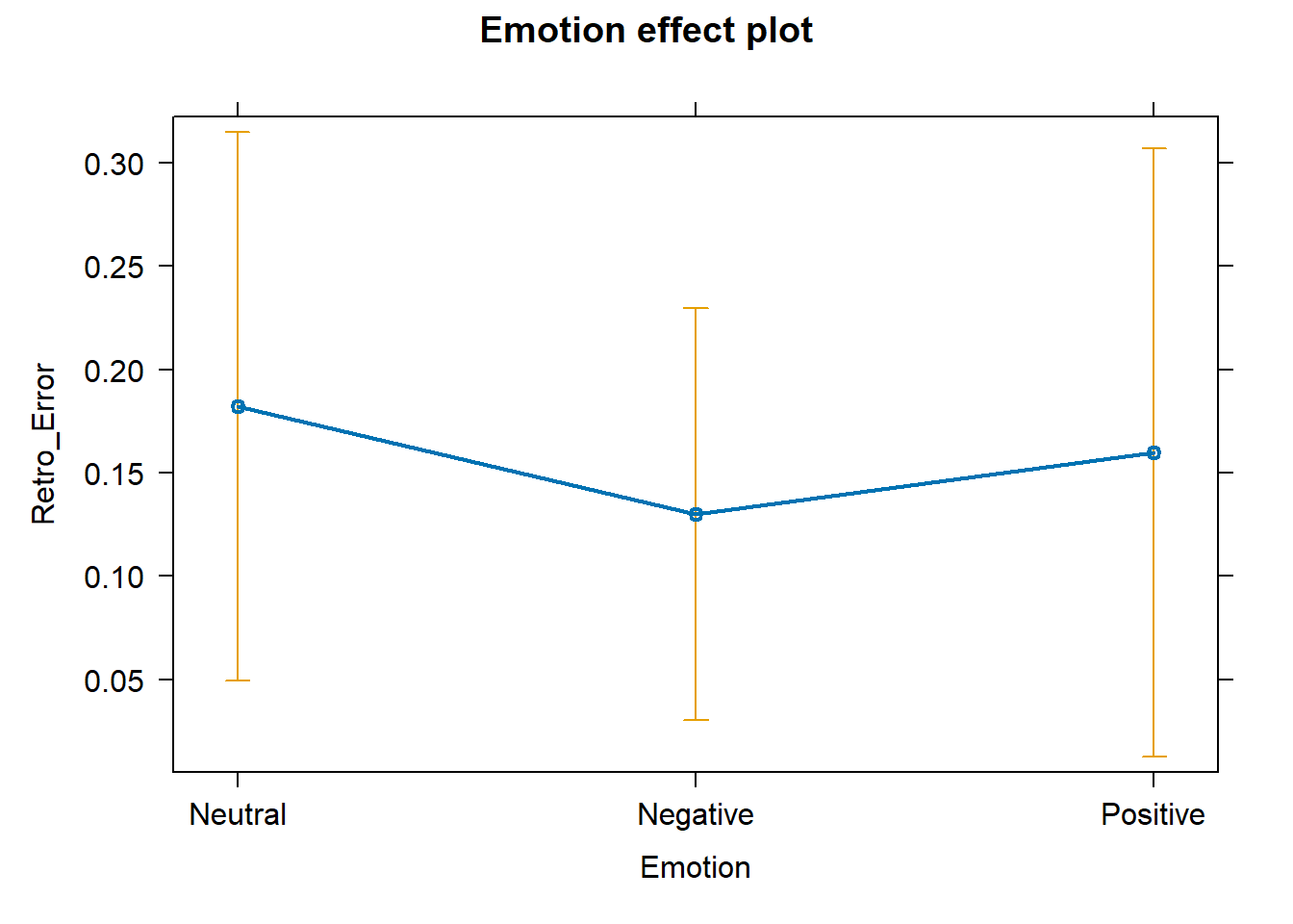
Retrospective Time

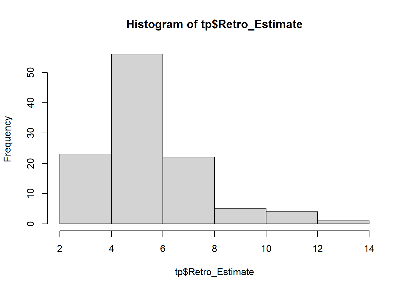
# inspect distribution of Retrospective estimates
hist(tp$Retro_Estimate)

Compute (in)accuracy as a ratio:

\[ RetrospectiveError = \frac{\text{Estimate} - \text{ObjectiveTime}}{\text{ObjectiveTime}} \]

# compute precision (error) of retrospective estimate
tp$Retro_Error = (tp$Retro_Estimate - 5) / 5

⮩ Positive values indicate overestimation. Negative values indicate underestimation.

But… if a video is largely overestimated by some and largely underestimated by others, the average error is zero… does it mean perfect accuracy? No! Global accuracy vs inaccuracy is reflected by the total amount of dispersion, while the average error indicates the tendency towards over- or under-estimation.

Fit Statistical Model on Retrospective estimates

# prepare factorial variables
tp$ID = factor(tp$ID)
tp$Emotion = factor(tp$Emotion, levels=c("Neutral","Negative","Positive"))

# actually fit the model
fit_re = glmmTMB(
  Retro_Error ~ Emotion + (1|ID),
  dispformula = ~ Emotion,
  data = tp
)

# see summary of model coefficients
summary(fit_re)

 Family: gaussian  ( identity )
Formula:          Retro_Error ~ Emotion + (1 | ID)
Dispersion:                   ~Emotion
Data: tp

     AIC      BIC   logLik deviance df.resid 
    73.2     92.2    -29.6     59.2      104 

Random effects:

Conditional model:
 Groups   Name        Variance Std.Dev.
 ID       (Intercept) 0.08629  0.2938  
 Residual                  NA      NA  
Number of obs: 111, groups:  ID, 37

Conditional model:
                Estimate Std. Error z value Pr(>|z|)   
(Intercept)      0.18216    0.06689   2.723  0.00646 **
EmotionNegative -0.05243    0.04835  -1.084  0.27819   
EmotionPositive -0.02243    0.07292  -0.308  0.75837   
---
Signif. codes:  0 '***' 0.001 '**' 0.01 '*' 0.05 '.' 0.1 ' ' 1

Dispersion model:
                Estimate Std. Error z value Pr(>|z|)    
(Intercept)      -2.5351     0.2562  -9.894   <2e-16 ***
EmotionNegative  -2.3919     1.4955  -1.599     0.11    
EmotionPositive   0.3938     0.3573   1.102     0.27    
---
Signif. codes:  0 '***' 0.001 '**' 0.01 '*' 0.05 '.' 0.1 ' ' 1

# plot predicted effects
plot(allEffects(fit_re))

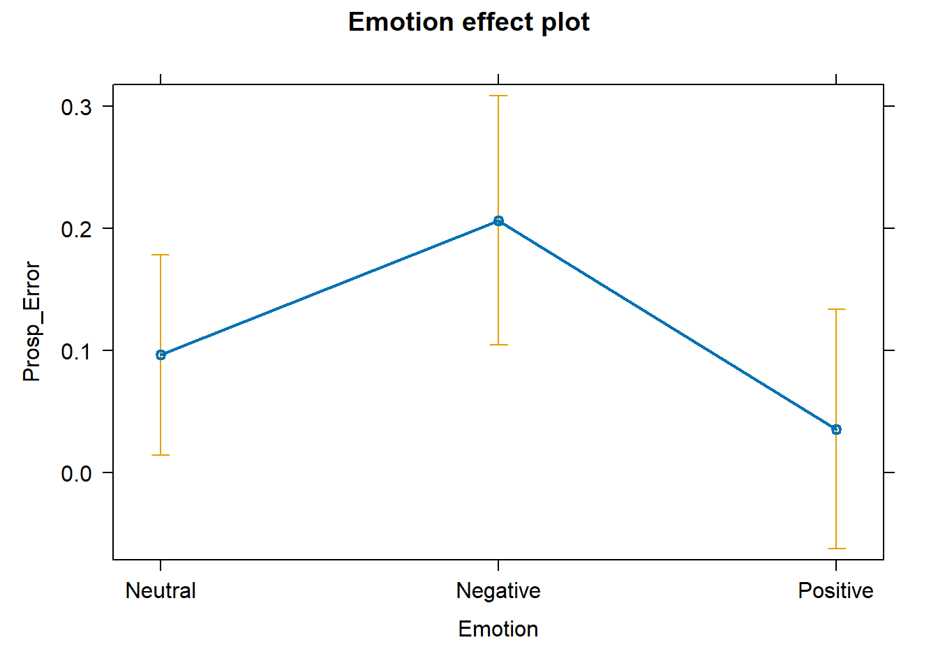
Prospective Time

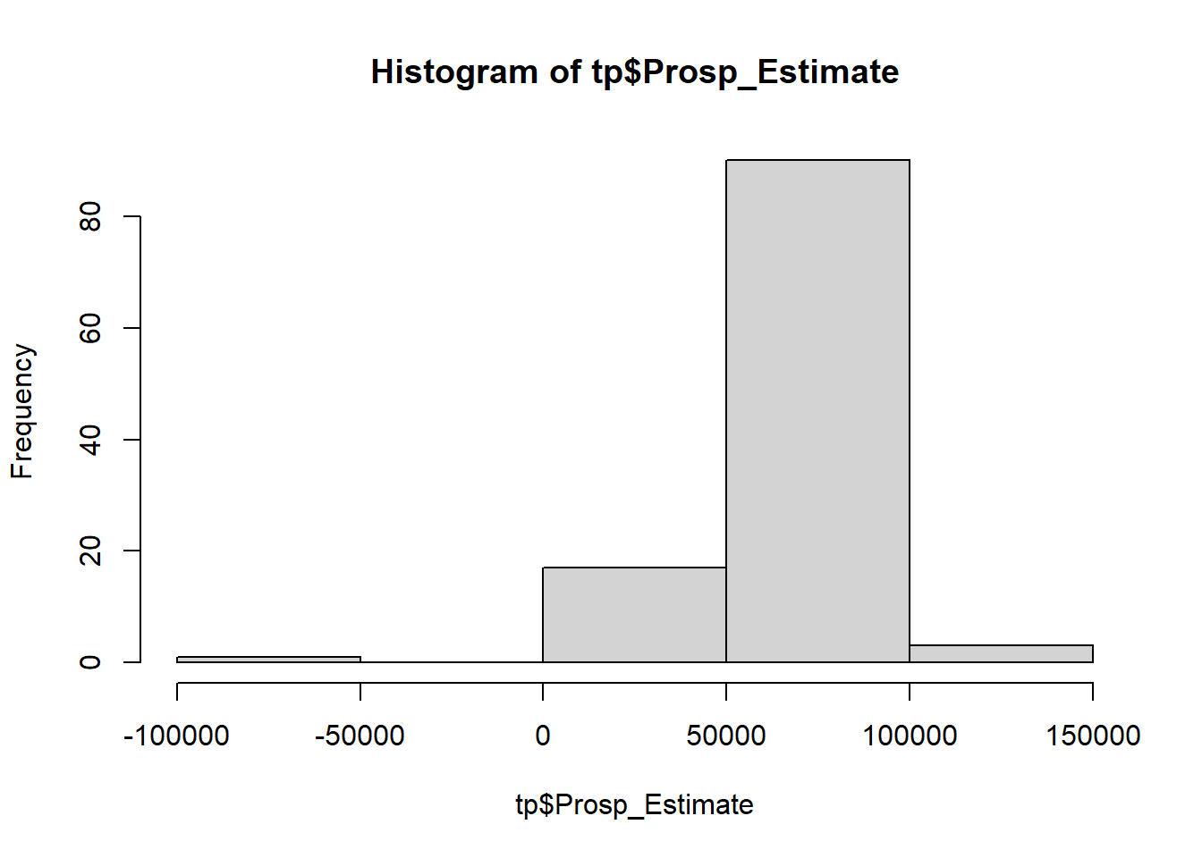
# inspect distribution of Prospective estimates
hist(tp$Prosp_Estimate)

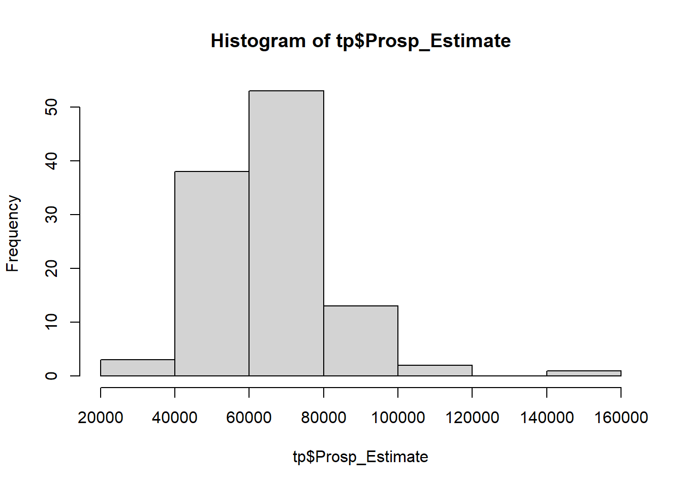
OUCH! There is a negative value! Remove it:

tp$Prosp_Estimate[tp$Prosp_Estimate < 0] = NA
hist(tp$Prosp_Estimate)

Compute error as a ratio:

\[ ProspectiveError = \frac{\text{Estimate} - \text{ObjectiveTime}}{\text{ObjectiveTime}} \]

# compute precision (error) of prospective estimate
tp$Prosp_Error = (tp$Prosp_Estimate - 60000) / 60000

Fit Statistical Model on Prospective estimates

fit_pro = glmmTMB(
  Prosp_Error ~ Emotion + (1|ID),
  dispformula = ~ Emotion,
  data = tp
)

# see summary of model coefficients
summary(fit_pro)

 Family: gaussian  ( identity )
Formula:          Prosp_Error ~ Emotion + (1 | ID)
Dispersion:                   ~Emotion
Data: tp

     AIC      BIC   logLik deviance df.resid 
     7.6     26.5      3.2     -6.4      103 

Random effects:

Conditional model:
 Groups   Name        Variance Std.Dev.
 ID       (Intercept) 0.05073  0.2252  
 Residual                  NA      NA  
Number of obs: 110, groups:  ID, 37

Conditional model:
                Estimate Std. Error z value Pr(>|z|)   
(Intercept)      0.09613    0.04133   2.326  0.02002 * 
EmotionNegative  0.11009    0.04019   2.739  0.00617 **
EmotionPositive -0.06066    0.03751  -1.617  0.10582   
---
Signif. codes:  0 '***' 0.001 '**' 0.01 '*' 0.05 '.' 0.1 ' ' 1

Dispersion model:
                Estimate Std. Error z value Pr(>|z|)    
(Intercept)      -4.3845     0.5722  -7.662 1.83e-14 ***
EmotionNegative   1.3005     0.6384   2.037   0.0417 *  
EmotionPositive   1.1552     0.7290   1.585   0.1131    
---
Signif. codes:  0 '***' 0.001 '**' 0.01 '*' 0.05 '.' 0.1 ' ' 1

# plot predicted effects
plot(allEffects(fit_pro))

Comments and Conclusions

For Finger tapping, it seems that Negative Emotion increases both average ITI and its dispersion within participants.
For the Retrospective task, it seems that Emotion has not particular effect on either estimation or its dispersion.
For the Prospective task, it seems that Emotion affects accuracy, causing both an average overestimation of duration in the Negative condition and some increase in its dispersion (absolute error).

An important point, when computing statistical analyses and finding relevant/significant effects, is to estimate how large they are. Since we used variables on interpretable metrics (ratio of error, milliseconds of ITI) the interpretation might be straightforward. However, standardized effect sizes (e.g., Cohen’s d) are also recommended.