Code
library(ggplot2)
source("R/simulationCode/N-and-k-Logistic.R")
library(ggplot2)
source("R/simulationCode/N-and-k-Logistic.R")In many cases, statistical power depends on more than one design feature simultaneously, for example sample size, number of trials per participant, and measurement reliability. When more than one of these features are free to vary, we need to explore multiple combinations that yield equivalent power. For example, one might aim to balance the number of participants and the number of trials per participant to find an optimal trade-off between recruitment effort and the experiment duration. This generalizes to many scenarios involving mixed-effects models, as you may need to allocate resources across multiple levels of grouping (e.g., children, schools, geographical regions).
The question is how the \(StdErr\)–based algorithm can be extended to handle multiple design parameters. To illustrate, we consider a mixed-effects logistic regression in which participants respond to multiple binomial trials. In this context, both an increase in sample size (\(N\)) and an increase in the number of trials per participant (\(k\)) can reduce the standard error of the effect of interest.
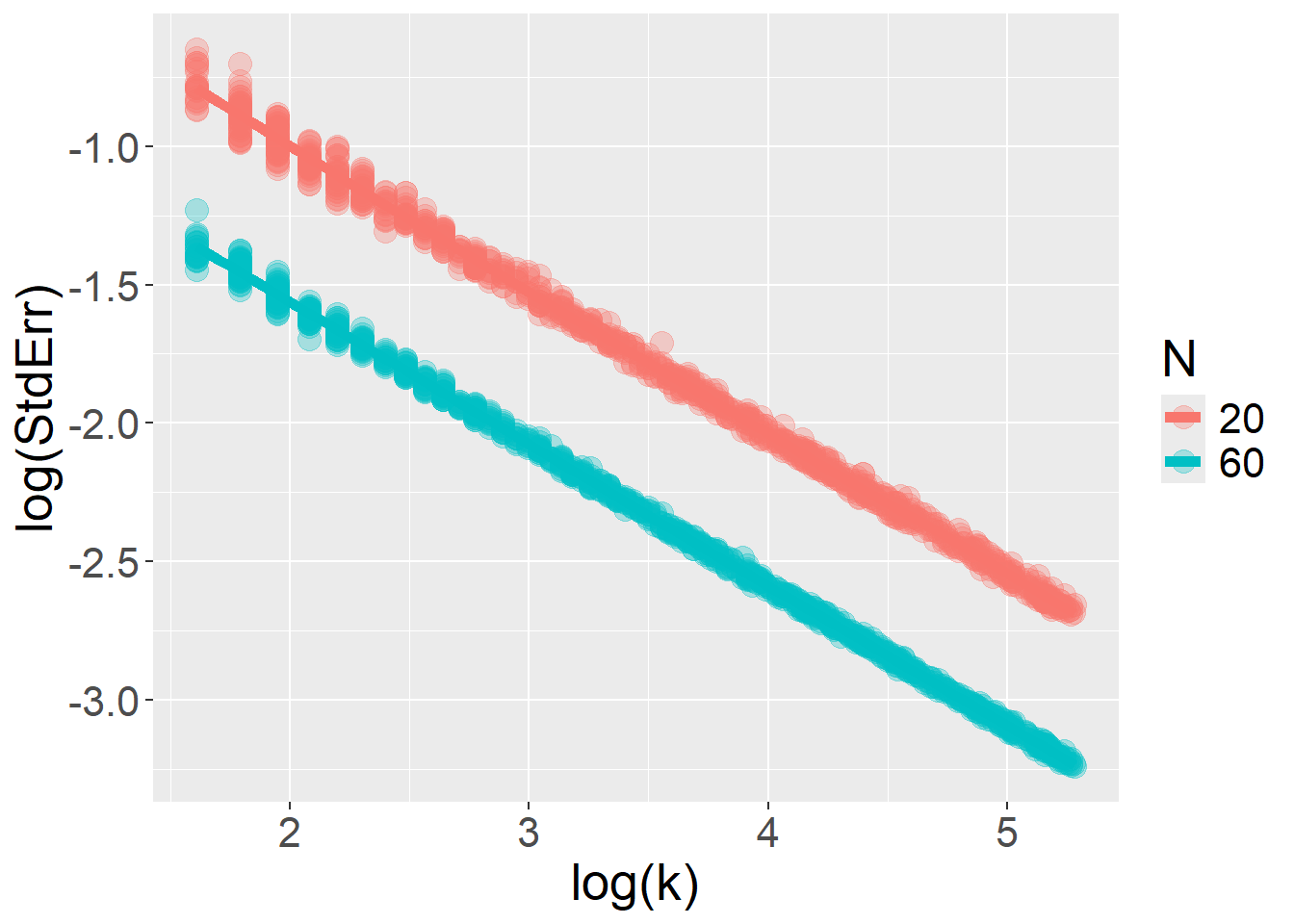
Can the algorithm be smoothly extended to \(k\), just as it is worked for \(N\)? Yes, but there are limitations. In many situations, \(StdErr\) does not continue to decrease indefinitely as a function of \(k\). This violates the log–log linearity between the number of observations and \(StdErr\). For a given value of \(N\), increasing \(k\) initially improves precision, but there is typically a point of diminishing returns, an asymptote beyond which collecting additional trials becomes practically useless for decreasing \(StdErr\).
glmer(response ~ group + (1|id), data=df,family = binomial(link="logit"))simData = function(N = 500, k = 10, tau = 0.8, B1 = 0){
require(lme4)
estimated_B=NA; SE=NA; p=NA
tryCatch({
# prepare random effects
rInts = rnorm(n=N, 0, tau)
rInt = rep(rInts, each=k)
id = rep(1:N, each=k)
# prepare fixed effects
group = rep(rbinom(N,1,0.5), each=k)
# generate linear component
yLinear =
0 +
B1*group +
rInt
# generate observed responses
response = rbinom(N*k, 1, prob=plogis(yLinear))
trial = rep(1:k, times=N)
# prepare dataset
df = data.frame(id, group, trial, response)
fit = glmer(response ~ group + (1|id), data=df, family = binomial(link="logit"))
su = summary(fit)
estimated_B = su$coefficients["group","Estimate"]
SE = su$coefficients["group","Std. Error"]
p = su$coefficients["group","Pr(>|z|)"]
},error=function(e){})
return(list(estimated_B=estimated_B,SE=SE,p=p))
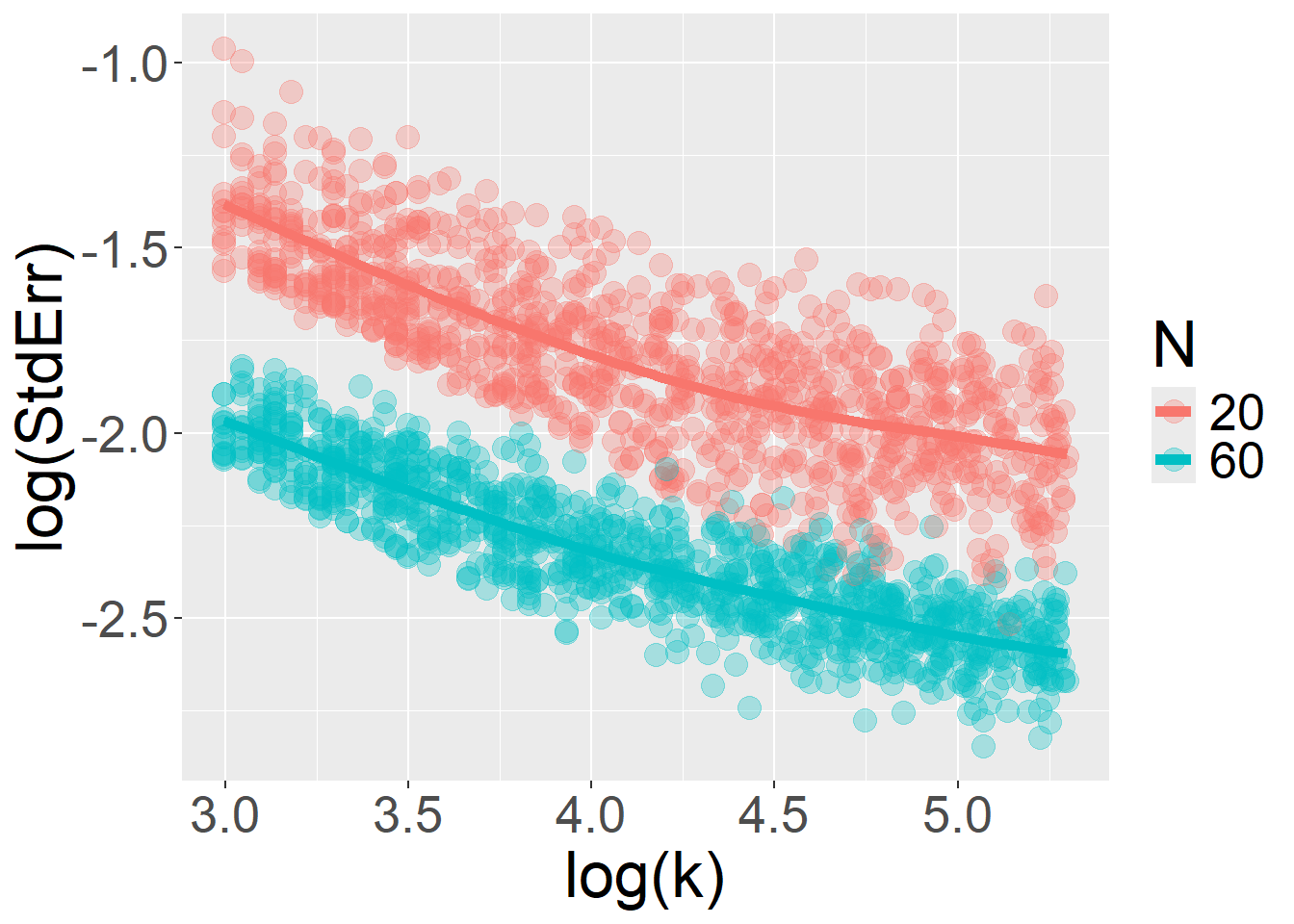
}This first case illustrates the core issue. Here, group is a categorical fixed effect that varies between participants, and response is a binary variable (say, performance on math items) modeled as a function of group membership (e.g., a special-needs group). In this setup, increasing the number of items (i.e., trials per participant, \(k\)) improves measurement precision and reduces \(StdErr\). However, the relationship between \(k\) and the standard error is not log–log linear.
For sample size \(N\), the expected log–log linear relationship with \(StdErr\) is quite obviously preserved:
But for the number of trials \(k\), the relationship breaks down and deviates from linearity:
glmer(response ~ type + (1|id), data=df,family = binomial(link="logit"))simData = function(N = 500, k = 10, tau = 0.8, B1 = 0){
require(lme4)
estimated_B=NA; SE=NA; p=NA
tryCatch({
# prepare random effects
rInts = rnorm(n=N, 0, tau)
rInt = rep(rInts, each=k)
id = rep(1:N, each=k)
# prepare fixed effects
type = rbinom(N*k,1,0.5)
# generate linear component
yLinear =
0 +
B1*type +
rInt
# generate observed responses
response = rbinom(N*k, 1, prob=plogis(yLinear))
trial = rep(1:k, times=N)
# prepare dataset
df = data.frame(id, type, trial, response)
fit = glmer(response ~ type + (1|id), data=df, family = binomial(link="logit"))
su = summary(fit)
estimated_B = su$coefficients["type","Estimate"]
SE = su$coefficients["type","Std. Error"]
p = su$coefficients["type","Pr(>|z|)"]
},error=function(e){})
return(list(estimated_B=estimated_B,SE=SE,p=p))
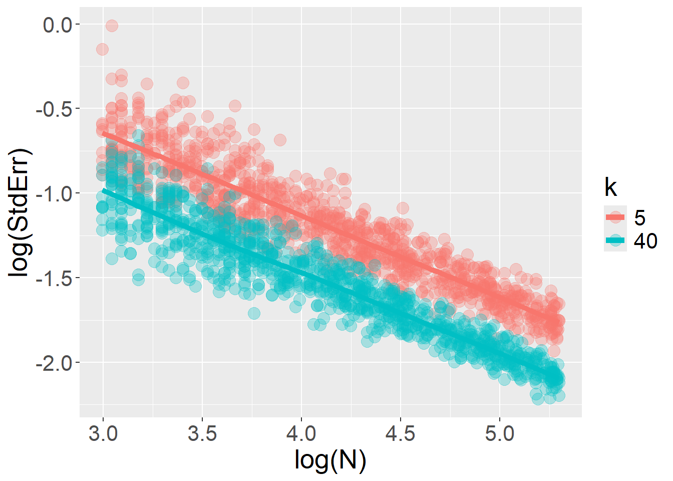
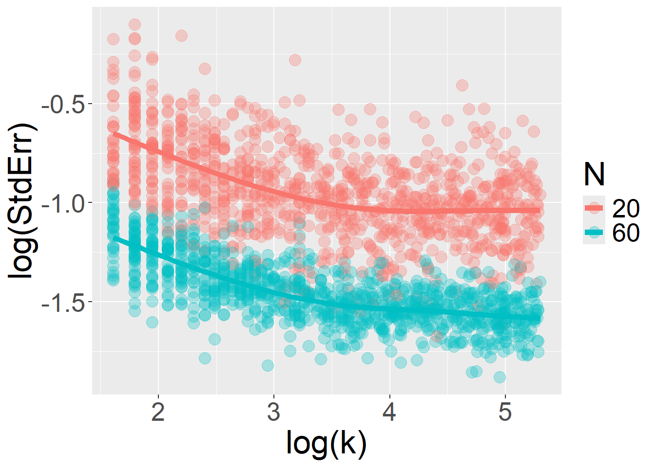
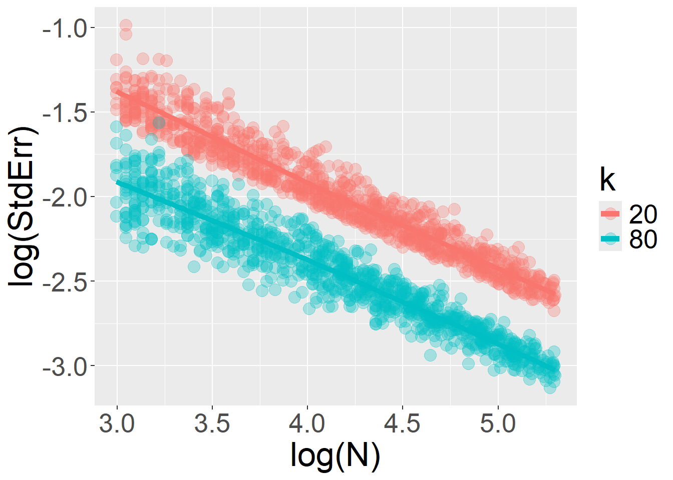
}The log–log relationship between \(StdErr\) and \(k\) is restored when the fixed effect (type) varies at the stimulus level, rather than across participants. In this scenario, increasing the number of trials accumulates more information without bound… but this is true only as long as the model includes only random intercepts and no random slopes.
For sample size \(N\):
For number of trials \(k\):
glmer(response ~ type + (type|id), data=df,family = binomial(link="logit"))simData = function(N = 500, k = 10, tau = 0.8, tauSlope = 0.5, B1 = 0){
require(lme4)
estimated_B=NA; SE=NA; p=NA
tryCatch({
# prepare random effects
rInts = rnorm(n=N, 0, tau)
rInt = rep(rInts, each=k)
rSlopes = rnorm(n=N, 0, tauSlope)
rSlo = rep(rSlopes, each=k)
id = rep(1:N, each=k)
# prepare fixed effects
type = rbinom(N*k,1,0.5)
# generate linear component
yLinear =
0 +
B1*type +
rInt +
rSlo*type
# generate observed responses
response = rbinom(N*k, 1, prob=plogis(yLinear))
trial = rep(1:k, times=N)
# prepare dataset
df = data.frame(id, type, trial, response)
fit = glmer(response ~ type + (type|id), data=df, family = binomial(link="logit"))
su = summary(fit)
estimated_B = su$coefficients["type","Estimate"]
SE = su$coefficients["type","Std. Error"]
p = su$coefficients["type","Pr(>|z|)"]
},error=function(e){})
return(list(estimated_B=estimated_B,SE=SE,p=p))
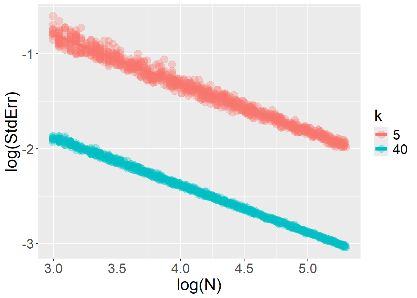
}Finally, when the model includes random slopes, increasing the number of trials per participant (\(k\)) no longer yields unlimited gains in precision. The sample size \(N\) becomes a limiting factor, and a ceiling is imposed on how much the \(StdErr\) can be further reduced by adding more trials \(k\).
For sample size \(N\):
For number of trials \(k\):