Basics of Data Science:
Numpy and Pandas

Enrico Toffalini

Why NumPy and Pandas?

Most data science pipelines in Python rely on these two packages, as base Python lacks built-in data structures like vectors with vectorized operations, matrices / arrays, and data frames

• numpy: efficient numerical computing (homogeneous arrays, vectorized operations) and many math, algebraic, and basic statistical functions;
• pandas: fundamental data structures for tabular data (DataFrames), with convenient indexing, reshaping, and data manipulation tools;

NumPy arrays

Remember the concept of “array” from Basics of R for Data Science?

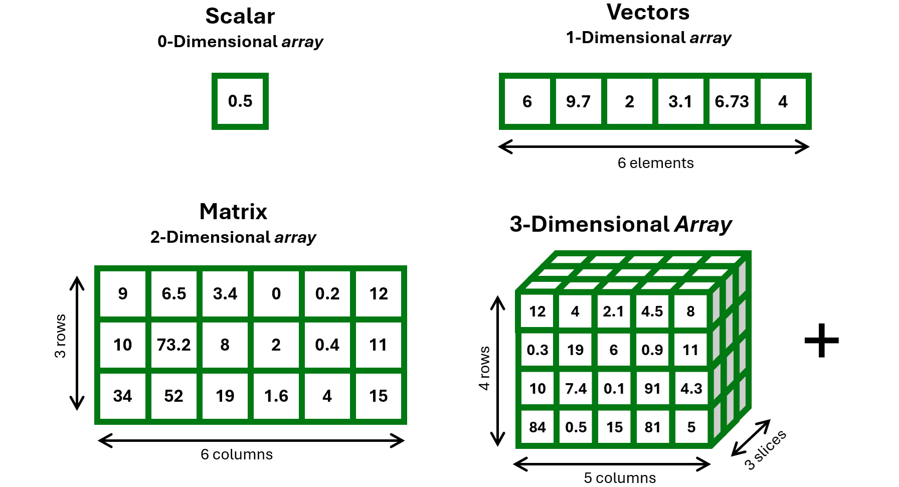
NumPy arrays

import numpy as np

Example of 1-D array

x = np.array( [6, 9.7, 2, 3.1, 6.73, 4] )
x

array([6.  , 9.7 , 2.  , 3.1 , 6.73, 4.  ])

Example of 2-D array (aka matrix, structured as a list of equally-long lists)

x = np.array( [[9, 6.5, 3.4, 0, 0.2, 12], 
               [10, 73.2, 8, 2, 0.4, 11], 
               [34, 52, 19,  1.6, 4, 15 ]] )
x

array([[ 9. ,  6.5,  3.4,  0. ,  0.2, 12. ],
       [10. , 73.2,  8. ,  2. ,  0.4, 11. ],
       [34. , 52. , 19. ,  1.6,  4. , 15. ]])

Arrays: Vectorized Operations

Unlike basic lists, arrays are homogenous and support fast vectorized operations, e.g., np.sqrt(x), x+5, x**2, etc.

x * 10

array([[ 90.,  65.,  34.,   0.,   2., 120.],
       [100., 732.,  80.,  20.,   4., 110.],
       [340., 520., 190.,  16.,  40., 150.]])

Different ways of doing the same thing:

np.round(np.sqrt(x), 4)

array([[3.    , 2.5495, 1.8439, 0.    , 0.4472, 3.4641],
       [3.1623, 8.5557, 2.8284, 1.4142, 0.6325, 3.3166],
       [5.831 , 7.2111, 4.3589, 1.2649, 2.    , 3.873 ]])

np.sqrt(x).round(4)

array([[3.    , 2.5495, 1.8439, 0.    , 0.4472, 3.4641],
       [3.1623, 8.5557, 2.8284, 1.4142, 0.6325, 3.3166],
       [5.831 , 7.2111, 4.3589, 1.2649, 2.    , 3.873 ]])

Arrays: Vectorized Operations

ar1 = np.array([1, 2, 3, 4])

ar2 = np.array([5, 6, 7, 8])

print(ar1 + ar2)       # element-wise addition

[ 6  8 10 12]

print(ar1 * ar2)       # element-wise multiplication

[ 5 12 21 32]

print(np.dot(ar1, ar2)) # dot product

70

These features make np.array() conceptually very similar to the c() and array() objects of R. However, as we will see, np.array() is stricter in enforcing data types

Arrays: Structural attributes

What you can inspect for an array:

x.shape    # tuple of sizes of dimensions

(3, 6)

x.ndim     # just the number of dimensions

2

x.size     # total number of elements

18

x.itemsize # memory size in bytes taken by a single element

8

x.nbytes   # total number of memory bytes occupied by the array

144

x.dtype    # data type of the array

dtype('float64')

Arrays: Data types

x = np.array([1.51, 2/3, 10, 14, 0.6])
x.dtype

dtype('float64')

x = np.array([24, 161, 10, 14, 188])
x.dtype

dtype('int64')

x = np.array(["aa","bb","cc","dd","❤❤"])
x.dtype

dtype('<U2')

x = np.array(["Hello world!","bb","cc","dd","❤❤"])
x.dtype

dtype('<U12')

x = np.array(["uselessly long string","bb","cc","dd","❤❤"])
x.dtype

dtype('<U21')

Arrays: Data type coercion

Python numpy

x = np.array([10,11,12,13,14])
x[0] = 3.14159
x

array([ 3, 11, 12, 13, 14])

R

x = c(10,11,12,13,14)
x[1] = 3.14159
x

[1]  3.14159 11.00000 12.00000 13.00000 14.00000

Even with characters!

x = np.array(["aa","bb","cc","dd","ee"])
x[0] = "Hello world!"
x

array(['He', 'bb', 'cc', 'dd', 'ee'], dtype='<U2')

x = c("aa","bb","cc","dd","ee")
x[1] = "Hello world!"
x

[1] "Hello world!" "bb"           "cc"           "dd"           "ee"          

😱

Arrays: Data type coercion

Actually, this “problem” is part of the secret of what makes Python numpy so efficient… but be careful!

How do you avoid this silent coercion? Explicitly state the data type from the beginning!

x = np.array([10,11,12,13,14], dtype="float64")
x[0] = 3.14159
x

array([ 3.14159, 11.     , 12.     , 13.     , 14.     ])

x = np.array(["aa","bb","cc","dd","ee"], dtype="<U40")
x[0] = "Hello world!"
x

array(['Hello world!', 'bb', 'cc', 'dd', 'ee'], dtype='<U40')

Arrays: Slicing and Indexing

x = np.array([10, 20, 30, 40, 50])
x[0]     # first element

np.int64(10)

x[-1]    # last element

np.int64(50)

x[1:4]   # elements 1 to 3

array([20, 30, 40])

x = np.array([[1,2,3,4], 
              [5,6,7,8]])
x[1,0]     # 2nd row, 1st column

np.int64(5)

x[-1,-1]   # last row, last column

np.int64(8)

x[0,]      # 1st row, all columns

array([1, 2, 3, 4])

Pandas Series

Series are essentially like 1D numpy arrays, but labelled with keys (numerical indexing is deprecated for Series)

import pandas as pd
grades = pd.Series([28, 15, 30, 23], index=["Jane", "Jim", "John", "Jack"])

print( grades["Jack"] )

23

print( grades[grades >= 18] )

Jane    28
John    30
Jack    23
dtype: int64

print( grades[["Jack","Jane"]] )

Jack    23
Jane    28
dtype: int64

Pandas DataFrame ❤️

pandas DataFrame is the classical tabular object we are familiar with; can be seen as a special type of Python dict (dictionary), composed of internally-homogeneous, equally-long, labelled lists

myDF = pd.DataFrame( {
    "teacher": ["Pastore", "Granziol", "Feraco", "Altoe", "Marci"],
    "course": ["CurrentIssues", "BasicsInference", "SEM", "Outliers", "QMP"],
    "hours": [10, 20, 20, 5, 5],
    "mandatory": [True, True, False, False, True],
    "semester": [1, 1, 2, 2, 2]
 } , index=["t1","t2","t3","t4","t5"])
myDF

     teacher           course  hours  mandatory  semester
t1   Pastore    CurrentIssues     10       True         1
t2  Granziol  BasicsInference     20       True         1
t3    Feraco              SEM     20      False         2
t4     Altoe         Outliers      5      False         2
t5     Marci              QMP      5       True         2

DataFrame: Inspecting

myDF.shape      # rows x columns

(5, 5)

myDF.columns    # column names

Index(['teacher', 'course', 'hours', 'mandatory', 'semester'], dtype='object')

myDF.info()     # structure

<class 'pandas.core.frame.DataFrame'>
Index: 5 entries, t1 to t5
Data columns (total 5 columns):
 #   Column     Non-Null Count  Dtype 
---  ------     --------------  ----- 
 0   teacher    5 non-null      object
 1   course     5 non-null      object
 2   hours      5 non-null      int64 
 3   mandatory  5 non-null      bool  
 4   semester   5 non-null      int64 
dtypes: bool(1), int64(2), object(2)
memory usage: 205.0+ bytes

myDF.dtypes     # data types

teacher      object
course       object
hours         int64
mandatory      bool
semester      int64
dtype: object

myDF.describe() # summary stats

           hours  semester
count   5.000000  5.000000
mean   12.000000  1.600000
std     7.582875  0.547723
min     5.000000  1.000000
25%     5.000000  1.000000
50%    10.000000  2.000000
75%    20.000000  2.000000
max    20.000000  2.000000

about equivalent to str() and summary() in R

DataFrame: Indexing columns

     teacher           course  hours  mandatory  semester
t1   Pastore    CurrentIssues     10       True         1
t2  Granziol  BasicsInference     20       True         1
t3    Feraco              SEM     20      False         2
t4     Altoe         Outliers      5      False         2
t5     Marci              QMP      5       True         2

Using general syntax: [ ]

myDF["teacher"]

t1     Pastore
t2    Granziol
t3      Feraco
t4       Altoe
t5       Marci
Name: teacher, dtype: object

Using dot notation

myDF.teacher 

t1     Pastore
t2    Granziol
t3      Feraco
t4       Altoe
t5       Marci
Name: teacher, dtype: object

DataFrame: Indexing columns + row slicing

     teacher           course  hours  mandatory  semester
t1   Pastore    CurrentIssues     10       True         1
t2  Granziol  BasicsInference     20       True         1
t3    Feraco              SEM     20      False         2
t4     Altoe         Outliers      5      False         2
t5     Marci              QMP      5       True         2

Combine column selection with row selection

myDF["teacher"][0:3]

t1     Pastore
t2    Granziol
t3      Feraco
Name: teacher, dtype: object

DataFrame: Indexing multiple columns

     teacher           course  hours  mandatory  semester
t1   Pastore    CurrentIssues     10       True         1
t2  Granziol  BasicsInference     20       True         1
t3    Feraco              SEM     20      False         2
t4     Altoe         Outliers      5      False         2
t5     Marci              QMP      5       True         2

Use a list of column names inside the brackets

myDF[["teacher","course"]]

     teacher           course
t1   Pastore    CurrentIssues
t2  Granziol  BasicsInference
t3    Feraco              SEM
t4     Altoe         Outliers
t5     Marci              QMP

DataFrame: Indexing columns + row slicing

     teacher           course  hours  mandatory  semester
t1   Pastore    CurrentIssues     10       True         1
t2  Granziol  BasicsInference     20       True         1
t3    Feraco              SEM     20      False         2
t4     Altoe         Outliers      5      False         2
t5     Marci              QMP      5       True         2

Combine column selection with row selection

myDF[["teacher","course"]][0:3]

     teacher           course
t1   Pastore    CurrentIssues
t2  Granziol  BasicsInference
t3    Feraco              SEM

DataFrame: Indexing rows

     teacher           course  hours  mandatory  semester
t1   Pastore    CurrentIssues     10       True         1
t2  Granziol  BasicsInference     20       True         1
t3    Feraco              SEM     20      False         2
t4     Altoe         Outliers      5      False         2
t5     Marci              QMP      5       True         2

Access rows by position

myDF.iloc[0]

teacher            Pastore
course       CurrentIssues
hours                   10
mandatory             True
semester                 1
Name: t1, dtype: object

Access rows by labels

myDF.loc["t1"]

teacher            Pastore
course       CurrentIssues
hours                   10
mandatory             True
semester                 1
Name: t1, dtype: object

DataFrame: Indexing multiple rows

     teacher           course  hours  mandatory  semester
t1   Pastore    CurrentIssues     10       True         1
t2  Granziol  BasicsInference     20       True         1
t3    Feraco              SEM     20      False         2
t4     Altoe         Outliers      5      False         2
t5     Marci              QMP      5       True         2

Access rows by position

myDF.iloc[0:2]

     teacher           course  hours  mandatory  semester
t1   Pastore    CurrentIssues     10       True         1
t2  Granziol  BasicsInference     20       True         1

Access rows by labels

myDF.loc[["t1","t2"]]

     teacher           course  hours  mandatory  semester
t1   Pastore    CurrentIssues     10       True         1
t2  Granziol  BasicsInference     20       True         1

DataFrame: Indexing rows + columns

     teacher           course  hours  mandatory  semester
t1   Pastore    CurrentIssues     10       True         1
t2  Granziol  BasicsInference     20       True         1
t3    Feraco              SEM     20      False         2
t4     Altoe         Outliers      5      False         2
t5     Marci              QMP      5       True         2

Access rows and columns

myDF.loc["t1", "teacher"]

'Pastore'

Access rows and columns

myDF.iloc[0, 0]

'Pastore'

this is very similar to indexing using myDF[0,0] or myDF[0,"teacher"] in R

DataFrame: Indexing rows + columns

If you don’t like the row index, drop it!

myDF = myDF.reset_index(drop=True)
myDF

    teacher           course  hours  mandatory  semester
0   Pastore    CurrentIssues     10       True         1
1  Granziol  BasicsInference     20       True         1
2    Feraco              SEM     20      False         2
3     Altoe         Outliers      5      False         2
4     Marci              QMP      5       True         2

myDF.loc[0, "teacher"]

'Pastore'

by default, rows have no names, and row names are not strictly needed in a DataFrame; without names, integer are used for indexing rows even using .loc[], which makes it more similar to R

DataFrame Logical indexing

    teacher           course  hours  mandatory  semester
0   Pastore    CurrentIssues     10       True         1
1  Granziol  BasicsInference     20       True         1
2    Feraco              SEM     20      False         2
3     Altoe         Outliers      5      False         2
4     Marci              QMP      5       True         2

myDF[ myDF["hours"] > 15 ]

    teacher           course  hours  mandatory  semester
1  Granziol  BasicsInference     20       True         1
2    Feraco              SEM     20      False         2

myDF[ myDF["teacher"] == "Pastore" ]

   teacher         course  hours  mandatory  semester
0  Pastore  CurrentIssues     10       True         1

myDF[ (myDF["hours"] > 5) & (myDF["mandatory"] == True) ]

    teacher           course  hours  mandatory  semester
0   Pastore    CurrentIssues     10       True         1
1  Granziol  BasicsInference     20       True         1

DataFrame Logical indexing

    teacher           course  hours  mandatory  semester
0   Pastore    CurrentIssues     10       True         1
1  Granziol  BasicsInference     20       True         1
2    Feraco              SEM     20      False         2
3     Altoe         Outliers      5      False         2
4     Marci              QMP      5       True         2

myDF[ myDF["hours"] > 15 ][["teacher","course"]]

    teacher           course
1  Granziol  BasicsInference
2    Feraco              SEM

myDF[ myDF["teacher"] == "Pastore" ][["teacher","course"]]

   teacher         course
0  Pastore  CurrentIssues

myDF[ (myDF["hours"] > 5) & (myDF["mandatory"] == True) ][["teacher","course"]]

    teacher           course
0   Pastore    CurrentIssues
1  Granziol  BasicsInference

DataFrame Logical indexing

    teacher           course  hours  mandatory  semester
0   Pastore    CurrentIssues     10       True         1
1  Granziol  BasicsInference     20       True         1
2    Feraco              SEM     20      False         2
3     Altoe         Outliers      5      False         2
4     Marci              QMP      5       True         2

myDF.loc[ myDF["hours"] > 15 , ["teacher","course"]]

    teacher           course
1  Granziol  BasicsInference
2    Feraco              SEM

myDF.loc[ myDF["teacher"] == "Pastore" , ["teacher","course"]]

   teacher         course
0  Pastore  CurrentIssues

myDF.loc[ (myDF["hours"] > 5) & (myDF["mandatory"] == True) , ["teacher","course"]]

    teacher           course
0   Pastore    CurrentIssues
1  Granziol  BasicsInference

Actually, this is the most recommended! especially for data manipulation

Add new Columns in a DataFrame

    teacher           course  hours  mandatory  semester
0   Pastore    CurrentIssues     10       True         1
1  Granziol  BasicsInference     20       True         1
2    Feraco              SEM     20      False         2
3     Altoe         Outliers      5      False         2
4     Marci              QMP      5       True         2

Just index a column that doesn’t exist… and fill it!

myDF["wellBoh"] = 10
myDF

    teacher           course  hours  mandatory  semester  wellBoh
0   Pastore    CurrentIssues     10       True         1       10
1  Granziol  BasicsInference     20       True         1       10
2    Feraco              SEM     20      False         2       10
3     Altoe         Outliers      5      False         2       10
4     Marci              QMP      5       True         2       10

Add new Columns in a DataFrame

    teacher           course  hours  mandatory  semester
0   Pastore    CurrentIssues     10       True         1
1  Granziol  BasicsInference     20       True         1
2    Feraco              SEM     20      False         2
3     Altoe         Outliers      5      False         2
4     Marci              QMP      5       True         2

Just index a column that doesn’t exist… and fill it!

myDF["wellBoh"] = np.random.normal(size=len(myDF)).round(3)
myDF

    teacher           course  hours  mandatory  semester  wellBoh
0   Pastore    CurrentIssues     10       True         1   -1.289
1  Granziol  BasicsInference     20       True         1    1.882
2    Feraco              SEM     20      False         2    1.099
3     Altoe         Outliers      5      False         2   -0.971
4     Marci              QMP      5       True         2    0.134

Modify Columns in a DataFrame

myDF["wellBoh"] = myDF["wellBoh"] + 50 
myDF

    teacher           course  hours  mandatory  semester  wellBoh
0   Pastore    CurrentIssues     10       True         1   48.711
1  Granziol  BasicsInference     20       True         1   51.882
2    Feraco              SEM     20      False         2   51.099
3     Altoe         Outliers      5      False         2   49.029
4     Marci              QMP      5       True         2   50.134

myDF.loc[myDF["hours"]>15, "wellBoh"] += 100000
myDF

    teacher           course  hours  mandatory  semester     wellBoh
0   Pastore    CurrentIssues     10       True         1      48.711
1  Granziol  BasicsInference     20       True         1  100051.882
2    Feraco              SEM     20      False         2  100051.099
3     Altoe         Outliers      5      False         2      49.029
4     Marci              QMP      5       True         2      50.134

DataFrame (Python pandas) vs data.frame (R)

Task	Python (pandas)	R
Select column	df["var"]	df["var"]
Select column	df.var	df$var
Multiple columns	df[["a", "b"]]	df[, c("a", "b")]
Filter rows	df[df["var"] > 0]	df[df$var > 0, ]
Add column	df["newVar"] = ...	df$newVar = ...
Modify column	df["var"] = df["var"]+10 df["var"] += 10	df$var = df$var+10
Summary	df.describe()	summary(df)
Row access	df.loc[0]	df[1, ]
Cell access	df.loc[0, "var"]	df[1, "var"]
Cell access	df.iloc[0, 2]	df[1, 3]

Merging DataFrames (with pd.merge())

df1 = pd.DataFrame({
  "ID": ["Jane", "Jim", "John", "Jack"],
  "department": ["dpg","dpg","dpss","dpss"],
  "age": [21.4, 22.5, 20.2, 23.0]
})
df1

     ID department   age
0  Jane        dpg  21.4
1   Jim        dpg  22.5
2  John       dpss  20.2
3  Jack       dpss  23.0

df2 = pd.DataFrame({
  "ID": ["Jim", "Jack", "John", "Jane"],
  "grade": [28, 15, 30, 23]
})
df2

     ID  grade
0   Jim     28
1  Jack     15
2  John     30
3  Jane     23

df = pd.merge(df1, df2, on="ID")
df

     ID department   age  grade
0  Jane        dpg  21.4     23
1   Jim        dpg  22.5     28
2  John       dpss  20.2     30
3  Jack       dpss  23.0     15

be careful! it will lose any row that does not match across both DataFrames by "name"! otherwise, add argument how="outer" to keep all values and possibly fill with NaN (missing values)

Concat. DataFrames (with pd.concat())

dfDPG = pd.DataFrame({
  "name": ["Jane", "Jim"],
  "grade": [28, 15],
  "department": ["dpg", "dpg"]
})
dfDPG

   name  grade department
0  Jane     28        dpg
1   Jim     15        dpg

dfDPSS = pd.DataFrame({
  "name": ["John", "Jack"],
  "grade": [30, 23],
  "department": ["dpss", "dpss"]
})
dfDPSS

   name  grade department
0  John     30       dpss
1  Jack     23       dpss

df = pd.concat([dfDPG, dfDPSS])
df

   name  grade department
0  Jane     28        dpg
1   Jim     15        dpg
0  John     30       dpss
1  Jack     23       dpss

this is much like rbind() in R, but using the argument axis may also work like the function cbind()

Reshape Wide → Long (with .melt())

dfWide = pd.DataFrame({
  "ID": ["id01", "id02", "id03"],
  "gender": ["m", "m", "f"],
  "T0": [-2.31, -1.70, -2.64],
  "T1": [-1.50, -0.86, -2.30]
})
dfWide

     ID gender    T0    T1
0  id01      m -2.31 -1.50
1  id02      m -1.70 -0.86
2  id03      f -2.64 -2.30

dfLong = dfWide.melt(id_vars=["ID","gender"], var_name="TIME", 
                                value_name="SCORE", value_vars=["T0","T1"])
dfLong

     ID gender TIME  SCORE
0  id01      m   T0  -2.31
1  id02      m   T0  -1.70
2  id03      f   T0  -2.64
3  id01      m   T1  -1.50
4  id02      m   T1  -0.86
5  id03      f   T1  -2.30

Reshape Long → Wide (with .pivot())

dfLong = pd.DataFrame({
  "ID": ["id01", "id01", "id02", "id02", "id03", "id03"],
  "gender": ["m", "m", "m", "m", "f", "f"],
  "TIME": ["T0", "T1", "T0", "T1", "T0", "T1"],
  "SCORE": [-2.31, -1.50, -1.70, -0.86, -2.64, -2.30]
}); dfLong

     ID gender TIME  SCORE
0  id01      m   T0  -2.31
1  id01      m   T1  -1.50
2  id02      m   T0  -1.70
3  id02      m   T1  -0.86
4  id03      f   T0  -2.64
5  id03      f   T1  -2.30

dfWide = dfLong.pivot(index=["ID","gender"], 
                           columns="TIME", values="SCORE").reset_index()
dfWide

TIME    ID gender    T0    T1
0     id01      m -2.31 -1.50
1     id02      m -1.70 -0.86
2     id03      f -2.64 -2.30

Grouped operations (with .groupby())

    teacher           course  hours  mandatory  semester     wellBoh
0   Pastore    CurrentIssues     10       True         1      48.711
1  Granziol  BasicsInference     20       True         1  100051.882
2    Feraco              SEM     20      False         2  100051.099
3     Altoe         Outliers      5      False         2      49.029
4     Marci              QMP      5       True         2      50.134

Count by group

myDF.groupby("mandatory").size()

mandatory
False    2
True     3
dtype: int64

Average or sum by group

myDF.groupby("semester")["hours"].mean()

semester
1    15.0
2    10.0
Name: hours, dtype: float64

Grouped operations (with .groupby())

Compute statistics for multiple columns by group

myDF.groupby("semester")[["hours","wellBoh"]].mean()

          hours       wellBoh
semester                     
1          15.0  50050.296500
2          10.0  33383.420667

myDF.groupby("semester")[["hours","wellBoh"]].std()

             hours       wellBoh
semester                        
1         7.071068  70712.920354
2         8.660254  57735.903051

Apply multiple functions with .agg()

myDF.agg({"hours": ["mean","std","min","max"],
          "wellBoh": ["mean","std","min","max"]
          }).round(2)

      hours    wellBoh
mean  12.00   40050.17
std    7.58   54773.46
min    5.00      48.71
max   20.00  100051.88

myDF.groupby("semester").agg({"hours": ["mean","std","min","max"],
                              "wellBoh": ["mean","std","min","max"]
                             }).round(2)

         hours                 wellBoh                            
          mean   std min max      mean       std    min        max
semester                                                          
1         15.0  7.07  10  20  50050.30  70712.92  48.71  100051.88
2         10.0  8.66   5  20  33383.42  57735.90  49.03  100051.10