python -m venv <nameOfVenv>Virtual Environments, Packages, Import/Export
Virtual Environments
Practically, they are local folders with an isolated Python environment. They contain:
- a full copy of the Python interpreter / a symlink to the main Python installation;
- all the packages you install at the exact versions used at that time
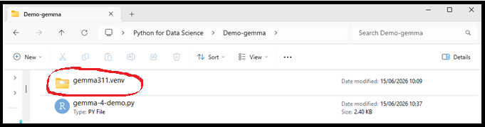
This folder is ideally placed inside your project directory
Virtual Environments
Create a virtual environment with this command in your bash/terminal:
then, just before using, activate it:
source <nameOfVenv>/bin/activate     # Linux/macOS

<nameOfVenv>\Scripts\activate        # Windows cmd / powershell
    # or alternatively
<nameOfVenv>\Scripts\activate.ps1    # Windows powershell
… from inside an IDE, you may activate the venv via specific commands like reticulate::use_virtualenv("nameOfMyVenv", required=T) (in R / RStudio), or setting the Python interpreter manually and then restarting the kernel (in Spyder)
Virtual Environments
- In your newly created
venv, you (re)install all packages required by your project. - Then, at any time, you can export a
requirements.txtfile to document the exact versions of all installed packages (this is particularly useful for sharing your environment, e.g., via GitHub). - This is best practice to isolate projects and ensure reproducibility.
pip freeze > requirements.txt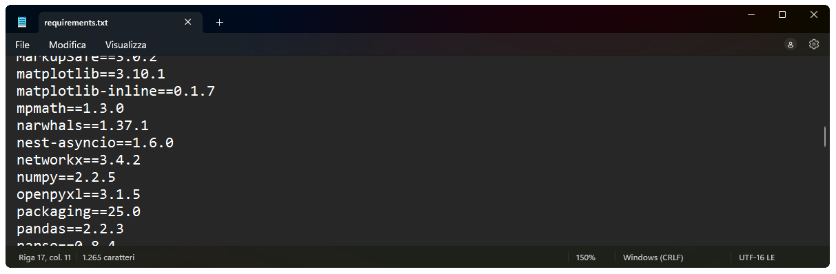
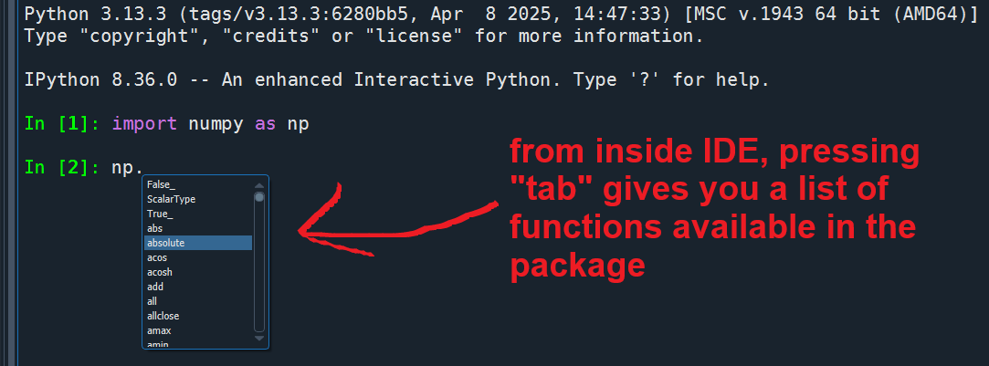
Using functions, help, autocomplete
Use a function from a package, and call help:
np.mean([2.0, 1.5, 7.1, 4.2]) # call a function from a package
?np.mean      # help only in IDE console or Colab,
help(np.mean) # help via built-in function
Use tab to autocomplete and explore available functions of a package ↴
Using functions, help, autocomplete
As in R, you can rely on positional order of arguments instead of naming them, or you can completely omit them if there are valid default arguments. However, it’s best practice to make all relevant arguments explicit for readability and reproducibility
sns.regplot(data=myDF, x="Age", y="Score", scatter=True, ci=95)
plt.show()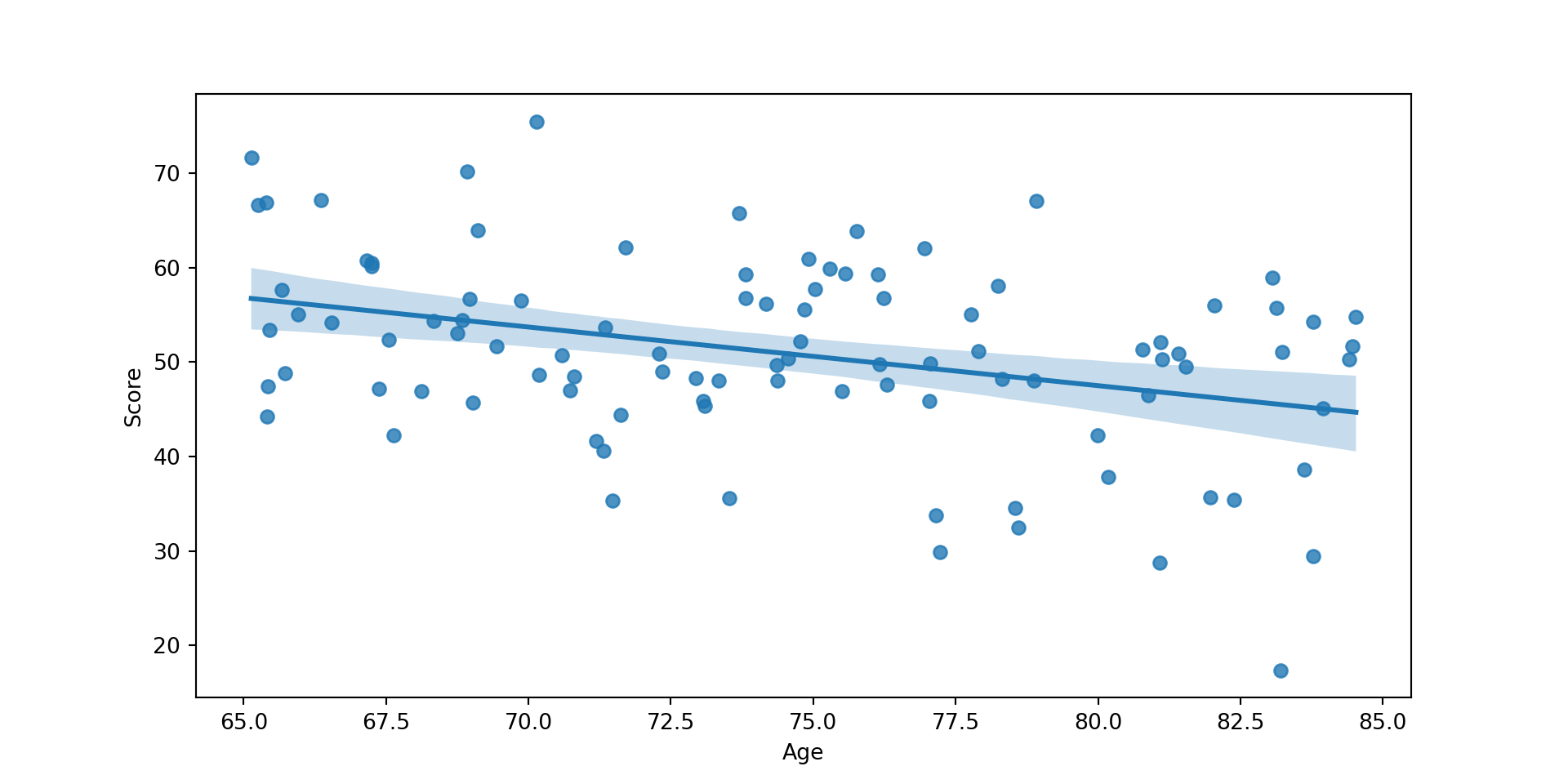
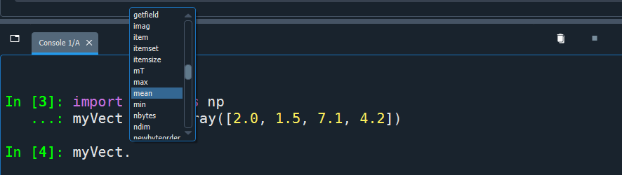
Accessing functions as methods
In Python, objects may have functions attached to them: these are called methods, and are accessed using dot (“.”) notation (more on this later!)
import numpy as np
myVect = np.array([2.0, 1.5, 7.1, 4.2])
Method-style syntax, requires that the object has this method:
myVect.mean()np.float64(3.7)
Function-style syntax
(more like R):
(more like R):
np.mean(myVect)np.float64(3.7)Use tab to autocomplete and explore available methods of an object →